 ,
which is plotted at the point between V2 and V1, or
,
which is plotted at the point between V2 and V1, or
 .
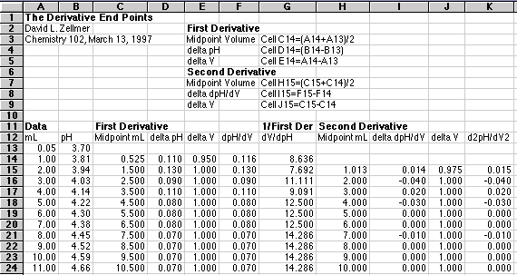
.The Derivative End Point Methods
©David L. Zellmer, Ph.D. |
Given two measurements in a pH vs. Volume plot: (V1, pH1) and (V2, pH2), the derivative is:
,
which is plotted at the point between V2 and V1, or
.
To compute the second derivative, just take the differences of the first derivative values, divide by the differences of the midpoint volumes and plot this at the point between the two midpoint volumes. The following spreadsheet example should make this clear.
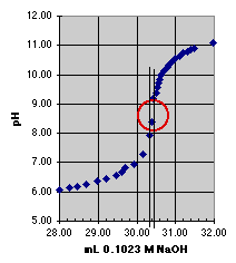
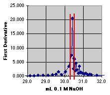
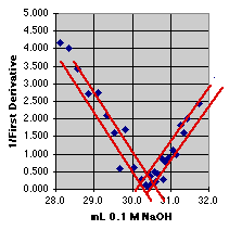
If our data were free of noise, these methods would give perfect results every time. The following graphs are from real student data. For each end point method used, we have to look at the graphs and estimate our best guess as to where the end point is, then estimate an error for each guess. Each plot below is in two forms: (1) a full plot of the entire curve, and (2) an expanded region where we can more easily make our end point estimates:
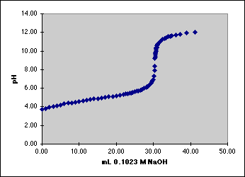
1. The "Eyeball" Method. Direct estimation from the titration curve.
|
|
Since error estimation must be done graphically, a larger plot than that shown above would be preferred. We can see, however, that the end point should lie somewhere within the circle we have drawn. There is a change in pH of about 2 units within this circle, but our estimated error comes from the change in volume within the circle, which is about 0.15 mL; so our estimated error is approximately plus or minus 0.07 mL. The end point volume is about 30.4 mL.
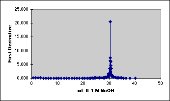
2. The First Derivative Method
|
|
At first glance, the first derivative method looks wonderfully precise. A sharp spike shows up right near 30 mL, just where we expect our end point. An expansion presents us with a dilemma, however. Had our data sample been just a hair different in pH, the position of the spike would have changed. The end point does appear to be at about 30.3 to 30.4 mL, but it could be as high as 30.5. We would probably estimate this one at 30.4 +or- 0.1 mL. (Again, a larger graph would make the estimate easier to see.)
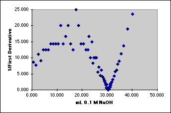
3. The Inverse First Derivative Method
|
|
The Inverse First Derivative (or 1/First Derivative) should trend toward zero as the derivative reaches a maximum. If there is a linear region near the end point, we may even be able to select some of these data and put a least squares line through them to estimate the end point. The expansion shows the problem. The noise in this real set of data makes the intersection quite uncertain. The end point seems to be at about 30.4 mL, +or- 0.3 mL(?).
4. The Second Derivative Method
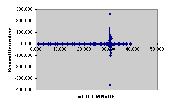
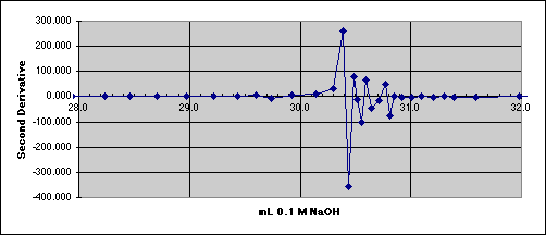
We need to reduce the noise.
All of these methods suffer from sensitivity to noise. Derivatives amplify noise, since they plot the rate of change of the signal. We observe in the lab that our meters become quite unstable right in the middle of our end point region. Methods such as Gran's Plotting take data from outside the noisy end point region, then average the responses by fitting a linear least squares line through the resulting plot. Other noise reduction methods include Sevitsky-Golay curve smoothing, a convolution method based on digital filtering and Fourier transform techniques. All of these methods belong to the larger field of Signal Processing, which has vast applications for science, industry, and military intelligence.
David L. Zellmer, Ph.D.This page was last updated on 13 March 1997
Department of Chemistry
California State University, Fresno
E-mail: david_zellmer@csufresno.edu