Gran's Plotting for End Point Detection
©David L. Zellmer, Ph.D. |
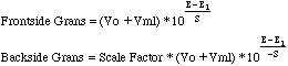
Gran's plotting is a method of end point detection that uses a linear decrease in the millimoles of chloride in the region well before the end point of the titration curve (Frontside Gran's). If the correct region is found, extrapolation to zero millimoles of chloride will intersect the volume axis at the end point. In the region following the end point, a similar linear plot of silver increase can also be extrapolated to the end point (Backside Gran's). The linearizing functions are based on the Nernst equation E=E1+S logC, where C is the molar concentration of the ion measured. S is the slope of the electrode used, typically +or- 59.2 mV for a univalent ion at 25o C. Solving for C and multiplying by the volume to get millimoles the functions become:
Vo is the initial volume of the solution in the titrated beaker. Vml is the volume added from the buret. E is the potential in millivolts. E1 is the first potential used in the Frontside Gran's Plot. A second value of E1 is used for the Backside plot. In the Backside case we choose the last value plotted. (I know this is confusing. Check out the Example below.) The Scale Factor in the Backside Gran's function is chosen to provide values that graph on the same chart as the Frontside values. The sign for the electrode slope S is reversed in the Backside equation. these differences between Front and Back arise from the fact that we first plot the decrease of the millimoles of Cl- on the Frontside, then we plot the increase in the millimoles of Ag+ on the backside. The concentrations of silver ion and chloride ion are inversely related through the Ksp expression.

This will all make a lot more sense when you actually try this on a spreadsheet.
To work up the data we have to:
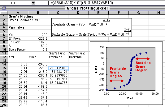
A portion of the E vs. Volume data is shown on this part of the spreadsheet. The Gran's regions are chosen from the parts of the curve that lie on either side of the end point. Don't approach too closely to the end point or the Gran's function will go non-linear. You can check this by plotting the Gran's function vs. volume and checking it for linearity. A common error that students make is to compute the Gran's function for the entire curve, and then wonder why they can't fit a straight line through it.
The formula for the first cell in the Gran's function is shown in the graphic above.
Cell C15=($B$6+A15)*10^((B15-$B$7)/$B$9)
When I first used this function I found that my values went UP as I approached the end point, rather than going down as they should. I fixed this by using a negative value for S, the slope of the electrode response. E1 Frontside is chosen as the first potential used in the Gran's function.
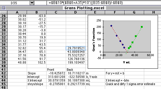
Cell D35=$B$10*($B$6+A35)*10^((B35-$B$8)/-$B$9)
The E1 value for this Backside plot is chosen from cell B39, the last E used in the function. When both functions were plotted on the same graph, the Backside plot was somewhat higher on the graph, so the Scale Factor was adjusted until both plots were about the same size on the graph. (Remember, first plot the Frontside Gran's vs. Volume, then use Paste Special... to paste the Backside series on top of the existing Frontside series.)
The data look linear, so we will proceed with the Linear Least Squares analysis. See the LLS tutorials elsewhere for details on how to do this. In this example:
Cell C42=SLOPE(C15:C19,A15:A19)
Cell C43=INTERCEPT(C15:C19,A15:A19)
Cell C44=-C43/C42
Cell C45=STEYX(C15:C19,A15:A19)/C42
The values for the Backside column are analogous.
The potentials plotted in this example contain small amounts of potential measurement error common to real analyses. The volume intercepts are near the ideal value of 30.00 mL, but not exactly equal to it. The Frontside value is 30.08 mL and the Backside value is 30.11 mL. Dividing the standard deviation about regression (STEYX()) by the slope gives us an estimate of the volume standard deviation, about +or- 0.28 mL for these plots. The data you use from the lab may contain a lot more error than this, giving rise to some pretty strange looking plots. It is common that the Gran's method fails on one side or the other of the end point.
By the way, a common student error is to place the end point where the Frontside and Backside plots cross each other. This is not correct. Each graph is a separate estimate of the end point, and uses the point where the plot crosses the volume axis.
The lines in the plot shown were created using the Trendline... command in Excel 5.0. Options allow you to select the kind of line used, and how far past the data the line extends so the volume axis can be crossed.
David L. Zellmer, Ph.D.This page was last updated on 3 March 1997
Department of Chemistry
California State University, Fresno
E-mail: david_zellmer@csufresno.edu