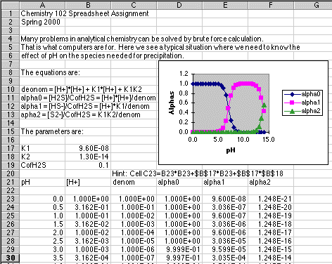
Your task is to duplicate the spreadsheet above.  Be careful to distinguish between values that have been entered by hand and those which have been calculated.  You will not receive credit for this assignment if you laboriously copy each and every number shown onto the spreadsheet!  (I have seen students do this.  It sort of defeats the purpose of using a computer, doesn't it?)

Here is how it was done:

The information in rows 1 through 13 is just text typed into the column A cell.  Such text is ignored by the computer but is useful to the humans reading the spreadsheet.

In cell A3 type Your Name and the current Date

In rows 15 through 19 we have a parameter block.  Labels are put in column A, and the corresponding numeric values are put in column B.  Note the use of the computer version of Scientific Notation used for the K values.  Excel does not support superscript and subscript in any useful fashion, so we have to write formulas in a way that is mostly readable.    becomes CofH2S, for example.

In row 21 we have labels for each quantity we wish to calculate.

In cell A23 we put our initial value of pH, in this case 0.
In cell A24 we put our first formula.  Type =A23+0.5 into cell A24, then press Enter.  Now click on this cell and drag it down to A51.  Choose Fill Down to generate all the other pH values automatically.  (Fill Down can be activated in a variety of ways, depending on the spreadsheet version you are using.  Ask your instructor or a friend.  Start by looking for Fill Down under the Edit Menu.  In the Mac version of Microsoft Excel 5.0 used in this example, it is found under Edit, then a Fill submenu with lots of options including creation of a series such as we just did with a formula.  Again, doing this with a mentor the first few times will save you a lot of time.  Just remember to WRITE DOWN any steps that you did not at first know how to do.)

In cell B23 put the formula =10^-A23.  This computes [H+] from pH.  Fill this down to cell B51.

In cell C23 put the formula =B23*B23+$B$17*B23+$B$17*$B$18.  Note the relative references such as B23, which point to the cell to the left of the formula which contains the [H+] it needs.  This reference will change as this formula is filled down.  $B$17, on the other hand, is an Absolute Reference and always points to the cell that contains the value of K1 needed in the calculation.

It is left as an exercise for the student to devise the formulas to put in the cells that generate alpha0, alpha1 and alpha2.

Format the numbers you have generated so they appear as shown.  pH uses the 0.0 format, and all the others use the 0.000E+00 format.  Select the numbers to be formated, then choose Format Number from the appropriate menu.  (Excel 5.0 has hidden this in dialog boxes found by choosing Format Cells... from the Format menu.)

Now that all of the values have been generated, it is time to produce the graph.  This is far easier to show on an actual compute than it is to give detailed written instructions, so don't hesitate to ask for help on this one.  Here are a few hints, however.

Although the data are evenly spaced, I still want you to use a Scatterplot when producing this graph.  Your X values will be in column A, and the three Y values to be plotted will be in columns D, E, and F.  This introduces a few complications.  You will probably need help getting this all to plot on your own computer, so don't hesitate to ask if you get stuck.

Here is how it worked in Microsoft Excel 5.0 on a Macintosh.

1. Use the mouse to select A23 to A51.

2. Hold down the Command Key and drag from D23 to F51.  All of the data you wish to plot should now be selected, with columnsA, D, E, and F selected, but B and C not selected.

3. Click on the Chart Wizard   in the tool bar.  Drag a box in the position shown for the spreadsheet graph.

4. Answer the questions that the Wizard gives you.  Select a Scatterplot with data points that are connected.  When the boxes come up that let you specify the axes, put pH on the X-axis, and Alphas on the Y axis. 

Note added January 2000: Putting the labels onto the Legend was a real trick using older versions of Excel like 5.0. If you are using Excel from Office 97 for the PC, or Office 98 for the Mac or Office 2000, the chart wizard will tell you when you can insert the Legend Labels of for Alpha0, Alpha1 and Alpha2. If you are using an older version of Excel, ask your instructor how to do this.

5. At the completion of the Wizard boxes you will have a usable graph.  A bit more cleaning up can be done by editing the graph itself. For example, you can change the way numbers are shown on an axis by clicking on the axis, then choosing Format/Selected Axis... from the Menubar.

6. Rather than making a small graph as was used to fit into the example, put your graph underneath your calculations, and drag it big enough to fill the width of the spreadsheet and tall enough to look good and show the features. If you can't see the details of your plot, it is too small.