|
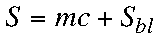
Sensitivity
S = signal from the instrument
m = sensitivity (slope of calibration curve)
c = concentration of analyte
Sbl = signal due to blank
|
|
|
Analytical Sensitivity
gamma = analytical sensitivity
m = sensitivity (slope of calibration curve)
ss = standard deviation of S
Note that increased instrumental gain will increase S, but will also increase Noise. Gamma will stay the same.
|

|
|
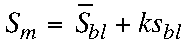
Detection Limit (signal)
Sm = minimum distinguishable signal
S-bar sub bl = mean blank signal
k = 3 (3 std deviations for 99% confidence)
sbl = std deviation of the blank signal
|
|
|
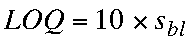
Limit of Quantitation (LOQ)
LOQ = lowest usable signal
sbl = std deviation of the blank signal
Note that this would give a relative standard deviation of 10%. Not great precision, but usable. |
|
|
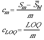
Detection Limit (analyte)
LOQ (analyte)
m = slope of Response vs. Concentration calibration curve
cm = analyte concentration corresponding to minimum signal. (See Sm above.)
c LOQ = analyte concentration corresponding to LOQ signal. (See LOQ above.)
|
|
|
Thermal (or Johnson) Noise
rms = root mean square
k = Boltzmann constant
T = temperature in kelvins
R = Resistance in ohms
delta f = instrument bandwidth
= 1/(3*rise time)
|
|
|
Shot Noise
I = average direct signal current
e = charge on electron
delta f = instrument bandwidth
|
|
|
Flicker Noise ("One over f")
Worse at lower frequencies (<100 Hz)
Also known as "drift" |

|
|
Signal Averaging
t = Student's t, about 1.96 for large N
s = standard deviation of the signal
N = number of signal samples
xbar = average signal over N samples
SHN uses different equations for signal averaging, but the result will be similar. Note that the Relative Standard Deviation = 100*s/xbar will overestimate the error for most real instruments, since some kind of filtering or signal averaging is used on the noisy signal. |
|
About significant figures: In the calculations below we will use the significant figures given by the computer in doing our calculations, just as you would do in the real world. Reported values, however, need to be rounded to the significant figures consistent with the errors. For example, the signal of 104.56 in the simulation below would be reported as 105 at best. Given that the 95% Confidence limit of a signal with a standard deviation of 20 and 100 signal samples would be about 1.96*20/sqrt(100) = 4, the reported value might be 105 +or- 4.
Simulated Signals and Noise
Simulations are useful tools for exploring how real instruments might operate. Be careful to distinguish between Parameters and Computed results. Parameters are the conditiions that we build into the simulation. They would be the "true" values that our measurements attempt to uncover. In the real world, the only values the instrument can give us are those found under Computed results in the spreadsheets below. We can use the simulated results to perform various statistical procedures in an attempt to uncover the "true" parameters.
The Microsoft Excel 5.0 spreadsheet was used to generate the values and graphs found below. Noise is added to the simulated signals using a modified random number generator that produces values with a gaussian distribution. The 200 element arrays containing the simulated data are not shown.
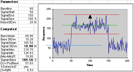
In the Parameters section of the spreadsheet we input the "true" values for our simulation. Under the Computed section we see the results of the simulation, just as we would have measured it on a real instrument. We first measure a baseline signal for 50 seconds, then introduce the analyte for 100 seconds, then return to the baseline for 50 more seconds. White noise with a gaussian distribution is added by the computer using a modified random number generator.
Noise is measured by sampling the baseline signal fifty times and taking the standard deviation. The value of 19.28 agrees well with the value of 20.0 set as a simulation parameter. The standard deviation of the signal itself is calculated in a similar way (100 samples), obtaining 18.90 for the Noise figure from the analyte signal itself. The mean baseline signal is 60.94 and the mean analyte signal is 165.50. The value of the signal above baseline is 165.50-60.94 = 104.56, a 4% departure from the value of 100 set in the simulation parameters--not great accuracy, but close to the 1-2% error expected from most instrumental methods.
Note that the size of the noise envelope (Max-Min) can be used to estimate the standard deviation of the signal. (Max-Min)/5 = 19.06, pretty close to the value of 20 set in the parameters.
The Detection Limit is computed at 3 x Std Dev of the baseline signal. For DL = 57.83 our signal of 104.56 is detected, so we could say that the analyte was indeed present. The Signal to Noise Ratio (S+N)/N is 6.53. Generally, SNR's of 2 to 3 are required to say we have detected a signal, so by this criterion we have detected our signal as well.
Our ability to measure this signal will be 4% using signal averaging over 100 samples (95% Confidence Limit = 1.96*18.90/sqrt(100) = 3.70; relative CL = 100*3.70/104.56 = 3.54%). Using the relative standard deviation (100*18.90/104.56 = 18.08) of 18% overestimates the error for most instuments using filtering or signal averaging.
Now consider the following smaller signal.
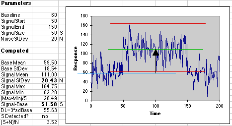
By the Detection Limit criterion we cannot say for sure that a signal is really present, even though our "eyeball" sees something there. The Signal to Noise is just over 3, so detection is possible. Clearly, this signal is at the edge of what we can detect.
If we use the "LOQ" criterion of 10 x the standard deviation of the baseline for our minimum useful signal, we would have a signal of about 200. Here's what this would look like:

Our error now is 100*(200-196.19)/200 = 1.91%, which is not bad, a bit better than the relative standard deviation of about 10%. Other measurements of this same signal will show the usual statistical fluctuations and may not be as good.
A really good signal of 500 would appear:
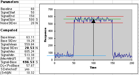
Here the difference between our parameter of 500 and our measured value of 496.5 is less than 1% of the signal measured. This would be a good result for most instrumental methods. The relative standard deviation is 100*20.53/500 = 4%, but signal averaging can reduce this substantially. If the signal is sampled 100 times, then averaged, the 95% Confidence Limit will be 20.53*1.96/sqrt(100) = 4.02, with a relative error of 100*4.02/500 = 0.80%, close to the error we found in the simulated result above.