Extended Statistics and Polynomial Fits with LINEST(Y-array,X-array,TRUE,TRUE) ©David L. Zellmer, Ph.D. Department of Chemistry California State University, Fresno

The Microsoft Excel function LINEST can generate many of the statistics we need when used in its full form.

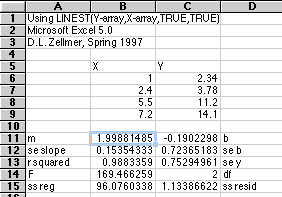
To generate the full array of statistics available with LINEST() we first select the block of cells from B11 to C15, then enter the formula =LINEST(C6:C9,B6:B9,TRUE,TRUE). Enter this array formula with Command+Enter (Mac) or Control+Shift+Enter (PC) and all the numbers shown in B11 to C15 will appear. The labels in columns A and D have been added afterwards for this presentation. The labels are those used in the HELP available in Excel.

Excel Label	Name	Equivalent Excel Function or Explanation
m	slope	=SLOPE()
se slope	standard error of the slope	This is the standard deviation of the slope, calculated in the tutorial on Equivalent Functions.
r squared	coefficient of determination	This is the famous number people quote to prove how good the fit is. It is quite useless for evaluating a working curve unless you count the "number of nines" you get. (0.978 is a pretty bad working curve. 0.999 is probably a good one.)
F	F-statistic	This is of little interest to an analytical chemist. If you're not sure that your instrument response is related to the concentration of the standards, you are in big trouble.
ss reg	regression sum of squares	See standard statistics texts.
b	intercept	=INTERCEPT()
se b	standard error of the intercept	This is the standard deviation of the Y-intercept. Use the functions for the error of a least-squares estimate when X=0 found in Equivalent Functions.
se y	standard error for the y estimate	=STEYX()
df	degrees of freedom	=COUNT()-2
ss resid	residual sum of squares	See standard statistics texts.

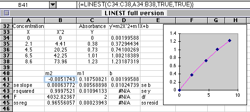
LINEST has one more surprise. It can do multiple regression, including polynomial fits. You have to do a little work yourself to make it perform. Lets say we want to fit the following Atomic Absorption working curve with a second order polynomial, y = m₂X² + m₁X + b, where y is the Absorbance observed, and X is the concentration of a standard.

You must observe the order shown above if you expect to plot out your results. Concentration goes in column A, the square of concentration goes in column B, and the resulting Absorbance in Column C. Then select the array B41:D45 and enter the equation =LINEST(C34:C38,A34:B38,TRUE,TRUE) and use Command+Enter (Mac) or Control+Shift+Enter (PC). The polynomial coefficients are found in row 41, with related statistics below. These coefficients are used to plot the values for the regression line in column D.

y' = -0.00517X² + 0.1875X + 0.0019996.

Using this multiple regression feature of LINEST you can fit any function you wish to your data, not just polynomials.

You can also use the TRENDLINE command to generate polynomial fits of any desired degree. Just plot out your function, plot it, click on the plot to select the data series, then choose Trendline... from the Insert menu. A dialog box lets you choose the function you want to fit. This Trendline... feature is found only in Excel 5.0 (Mac version number) or later, while the full LINEST is found in Excel 3.0 or later.

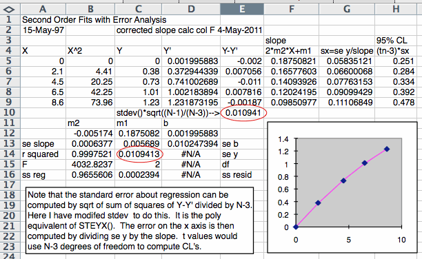
In other parts of this tutorial we have used the standard deviation about regression STEYX() to calculate the error when using a working curve fitted with a straight line. The second order polynomial fit equivalent of this is the value se y generated by the full LINEST output. Students who have used TRENDLINE... or other programs to do a second order fit can calculate this statistic by taking the "standard deviation" of Y-Y', where Y' is the regression line calculated from Y' = m2*X^2+m1*X+b. The normal function for STDEV() must be modified to reflect N-3 degrees of freedom instead of N-1 degrees of freedom. The spreadsheet below illustrates how we can do this. Both the LINEST method and the Y-Y' method are shown in this example.

This example also shows how we compute the errors on the X-axis. The X-axis would typically be a concentration if this is a working curve. The error in X is the error in Y divided by the slope. Since the slope varies from point to point in a second order fit, we compute the derivative of the function and compute that at each X value. Finally, we compute a 95% Confidence Limit uncertainty at each X value by using TINV(0.05,N-3), again using N-3 degrees of freedom.