It is an indeterminate form of type 0/0. There are several approaches (some of which were discussed in Math 75). First define Define f[x_]=(x+Tan[x])/Sin[x];
Introduction to Mathematica
For Math 76, Mathematical Analysis II
Remember to use Shift + Enter to process your inputs.
Plot the graphs of the exponential and logarithmic functions with base 1.5, that is, 1.5x and log1.5x, on the same coordinate system, e.g. type
Plot[{1.5^x, Log[1.5,x]}, {x,-10,10}]. You get some error messages. Why?
It is hard to see how the two graphs are related because the range of y is different from that of x. To make the graph easier to study, try
Plot[{1.5^x, Log[1.5,x]}, {x,-10,10}, PlotRange->{-10,10}, AspectRatio->1].
Notice that the two graphs are reflections of each other about the line y=x.
Exercise: Add the line y=x to the above graphs.
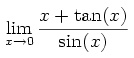
Consider the limit
It is an indeterminate form of type 0/0. There are several approaches (some of which were discussed in Math 75). First define Define f[x_]=(x+Tan[x])/Sin[x];
Exercise: Explore and compute the following limits:
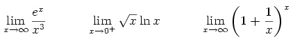
Note: For x approaching infinity, type x->Infinity.
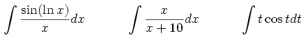
To find the indefinite integral (an antiderivative) of a function f(x), use Integrate[f[x],x].
Exercise: Try the following and explain the results you get:
Integrate[E^x,x]
Integrate[e^x,x]
Exercise: Evaluate the following integrals by hand first and then use Mathematica to check your answers:
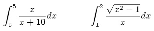
To evaluate the definite integral of a function f(x) from a to b, use Integrate[f[x],{x,a,b}], or NIntegrate[f[x],{x,a,b}] to get a numerical answer. For example, Integrate[Cos[x],{x,1,2}] gives sin(2)-sin(1), and NIntegrate[Cos[x],{x,1,2}] gives 0.0678264.
Exercise: Evaluate the following integrals by hand first and then use Mathematica to check your answers:
Exercise: Try the following and explain the relults you get:
Integrate[E^Sin[1/x],x]
NIntegrate[E^Sin[1/x],{x,1,2}]
NIntegrate[E^Sin[1/x],{x,0,2}]. To explain the warning messages, try graphing the function from 0 to 2.
Extra exercise: Answer the following questions without using Mathematica first, and then use Mathematica to check your answers.
Use DSolve[equation, y[x], x], e.g. DSolve[y'[x]==3y[x], y[x], x]
or DSolve[y''[x]+y[x]==0, y[x], x].
To find the solution that satisfies initial condition(s), write the equation and the condition(s) in curly brackets,
e.g. DSolve[{y'[x]==3y[x], y[0]==2}, y[x], x]
or DSolve[{y''[x]+y[x]==0, y[0]==3, y'[0]==4}, y[x], x].
Exercise: Solve the equation: y'+y=sin(x)+3.
Exercise: Solve the initial value problem: y'+y=sin(x)+3, y(0)=1.
Try the following:
solution=NDSolve[{y'''[x]+y''[x]+y'[x]==-(y[x])^3, y[0]==1, y'[0]==0, y''[0]==0}, y[x], {x,0,20}];
Plot[y[x]/.solution, {x,0,20}]
It will graph the solution of y'''(x)+y''(x)+y'(x)=-(y(x))^3 satisfying y(0)=1, y'(0)=0, y''(0)=0.
Exercise: Plot the solution of the initial value problem: y'=y-x3, y(0)=2, for x in [0,5].
Use ParametricPlot[{f[t],g[t]},{t,min,max}] to plot the curve given by x=f(t), y=g(t), for t in the interval [min,max]. Sometimes Mathematica gets upset (I don't really know why), and you have to use "Evaluate" as follows: ParametricPlot[Evaluate[{f[t],g[t]}],{t,min,max}].
Plot the curve given by x=t3+t2, y=1-t2, for t in the interval [-5,5]. Also plot this curve for t in the interval [-50,50].
Just as when plotting the graph of a regular function, you can define f(t) and g(t) first. So you can do the above as follows:
f[t_]=t^3-t^2;
g[t_]=1-t^2;
ParametricPlot[{f[t],g[t]},{t,-5,5}]
ParametricPlot[{f[t],g[t]},{t,-50,50}]
Exercise:
Exercise:
Project due November 3, 2004, at 11:59 pm:
Note 1: Collaboration is allowed, however, every person is expected to type and submit their own work.
Note 2: If you make a typo, please fix it instead of trying all over again. If you don't see what you typed wrong and wish to rewrite the whole thing, then erase the command that did
not work.
Open a new Mathematica file and write your name.
Consider the cycloid given by parametric equations x=t-sin(t), y=1-cos(t) (See example 6 on pages 690-691, let r=1).